add_figure

run.add_figure(key, figure, step=None, *, time=None)

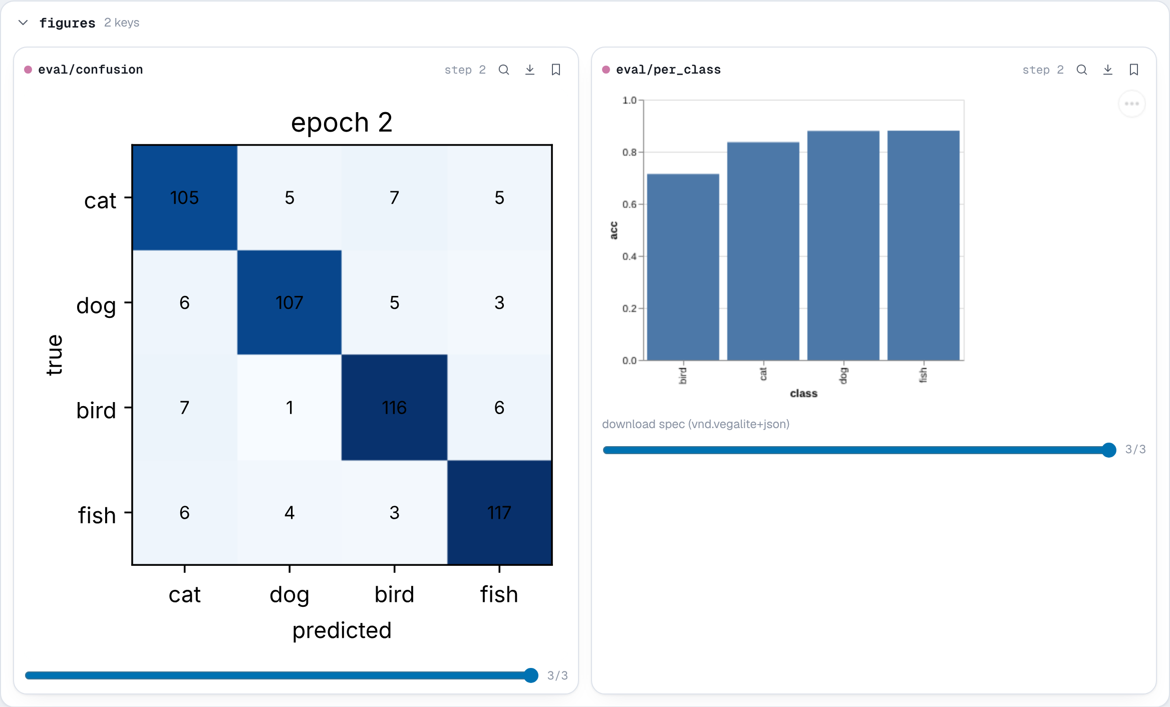
Logs a chart made with a plotting library: a confusion matrix, a per-class bar chart, a learning-rate schedule, or anything else a line chart does not cover.

Parameters

• key (str): the name the figure is logged under.
• figure: one of
  • a matplotlib figure, or the matplotlib.pyplot module for the current figure;
  • a Plotly figure, or a Plotly figure dict ({"data": [...], "layout": {...}});
  • an Altair chart, or a Vega-Lite spec as a dict with a $schema;
  • a Bokeh figure or layout;
  • a nb.WaveformFigure: audio with signals drawn over its waveform.
• step (int, optional): the training step.

Stored as the figure's own serialized form: Plotly JSON, a Vega-Lite spec or a Bokeh JSON item, and SVG for matplotlib. The figure is serialized on the calling thread, since figures are mutable, with the library that made it. NuBoard depends on none of these libraries, and plain dicts work without any of them.

In the viewer Plotly, Vega-Lite and Bokeh figures stay interactive (hover, zoom, pan), each in its own sandboxed frame, and follow the light or dark theme. Plotly and Vega-Lite are bundled with the viewer, so they work offline. Bokeh loads BokehJS from its CDN, for the exact version that wrote the figure. Matplotlib figures show as images. Figures are listed under Figures.

Example

import matplotlib

matplotlib.use("Agg")
import matplotlib.pyplot as plt
import numpy as np

import nuboard as nb

classes = ["cat", "dog", "bird", "fish"]
run = nb.init("api-tour", run_name="figures")
rng = np.random.default_rng(0)

for epoch in range(3):
    acc = 0.55 + 0.12 * epoch
    cm = rng.integers(1, 8, (4, 4)) + np.diag(rng.integers(30, 40, 4)) * (1 + epoch)

    fig, ax = plt.subplots(figsize=(4, 3.4))
    ax.imshow(cm, cmap="Blues")
    ax.set(xticks=range(4), yticks=range(4), xticklabels=classes, yticklabels=classes)
    ax.set(xlabel="predicted", ylabel="true", title=f"epoch {epoch}")
    for i, j in np.ndindex(cm.shape):
        ax.text(j, i, cm[i, j], ha="center", va="center", fontsize=8)
    run.add_figure("eval/confusion", fig, step=epoch)
    plt.close(fig)

    per_class = [{"class": c, "acc": round(acc + rng.normal(0, 0.06), 3)} for c in classes]
    run.add_figure(
        "eval/per_class",
        {
            "$schema": "https://vega.github.io/schema/vega-lite/v6.json",
            "data": {"values": per_class},
            "width": 320,
            "height": 260,
            "mark": "bar",
            "encoding": {
                "x": {"field": "class", "type": "nominal"},
                "y": {"field": "acc", "type": "quantitative", "scale": {"domain": [0, 1]}},
            },
        },
        step=epoch,
    )

run.finish()

The same chart from each library:

PlotlyAltairBokehmatplotlib

import plotly.express as px

fig = px.bar(x=classes, y=accs, labels={"x": "class", "y": "acc"})
run.add_figure("eval/per_class", fig, step=epoch)

import altair as alt
import pandas as pd

chart = (
    alt.Chart(pd.DataFrame({"class": classes, "acc": accs})).mark_bar().encode(x="class", y="acc")
)
run.add_figure("eval/per_class", chart, step=epoch)

from bokeh.plotting import figure

fig = figure(x_range=classes, height=300)
fig.vbar(x=classes, top=accs, width=0.8)
run.add_figure("eval/per_class", fig, step=epoch)

fig, ax = plt.subplots()
ax.bar(classes, accs)
run.add_figure("eval/per_class", fig, step=epoch)

Expected result

Waveforms with signals

nb.WaveformFigure(audio, sample_rate, signals, *, range=None, regions=None, caption=None)

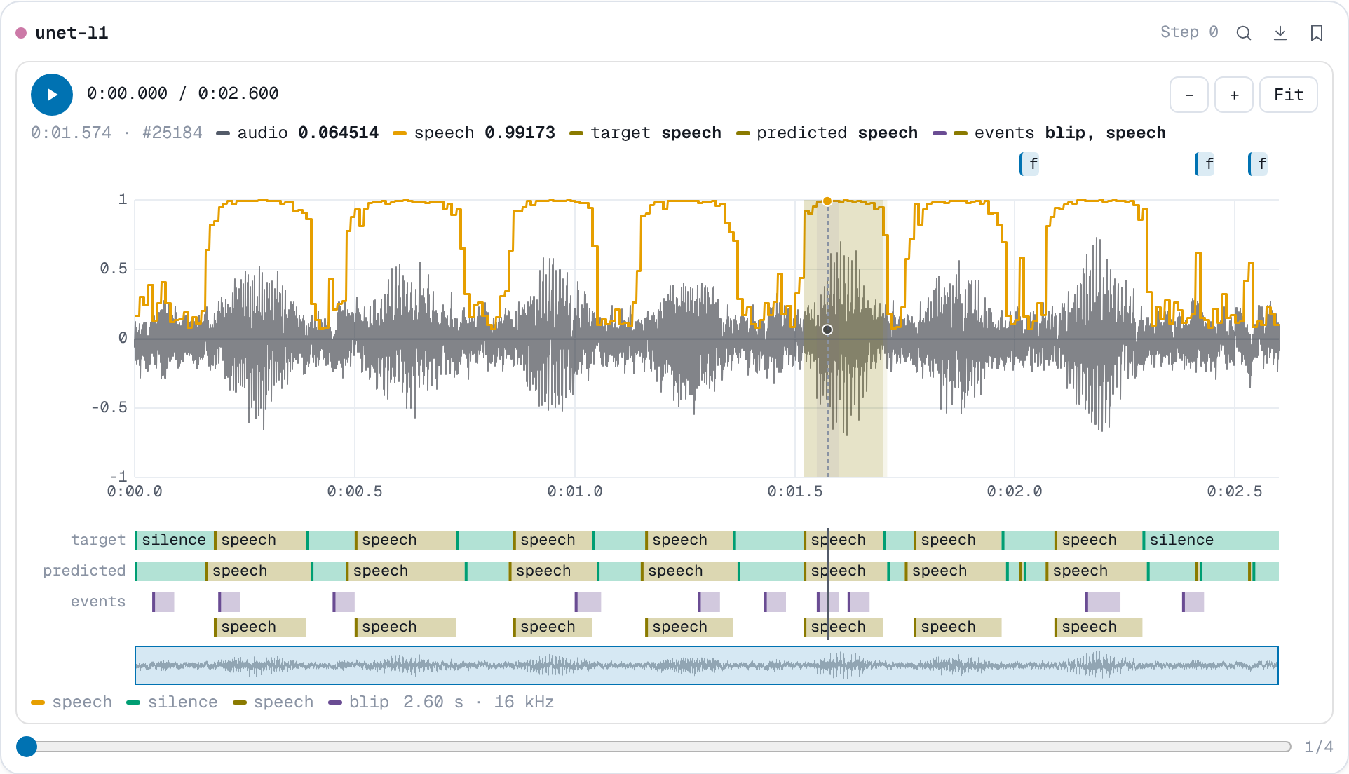
A figure made by NuBoard itself: a waveform with signals drawn over it, such as a voice activity probability, a gain mask or an envelope, one value per audio sample, and optionally labelled time regions, such as a classifier's target and predicted classes. It needs no plotting library, only NumPy for the arrays.

Parameters

• audio: a (samples,) or (channels, samples) array or tensor, read as add_audio reads it.
• sample_rate (int): samples per second.
• signals: an array or tensor of one value per audio sample, or a dict of them by name. A signal of the wrong length raises ValueError when it is logged. NaN leaves a gap.
• range (tuple, optional): the values at the bottom and top of the plot. Defaults to the waveform's own axis, -1 to 1 (full scale), so a signal shares the waveform's scale: an envelope traces it and a probability of 1 reaches the top. With a range, the signals get their own axis on the right.

• regions (dict, optional): labelled time regions logged with the figure, as tracks by name. Each track is one of

  • a list of (start, end, label) in seconds, which may overlap;
  • (ids, names, frame): a class id per frame (1-D), the class names and the frame length in seconds, as a single-label classifier outputs it;
  • (multi_hot, names, frame): a (frames, classes) array of 0 and 1, for classes that can be on at the same time (multi-label).

  Consecutive frames of one class are stored as one segment, so an hour of 10 ms frames stays small. A malformed track raises ValueError when it is logged. - caption (str, optional): a caption shown under the plot.

range, regions and caption are keyword-only.

A model that outputs one value per frame repeats it over the frame's samples:

probs = vad(wav)  # one speech probability per 10 ms frame at 16 kHz
signal = np.repeat(probs, 160)[: len(wav)]
run.add_figure("eval/vad", nb.WaveformFigure(wav, 16_000, {"vad": signal}), step=epoch)

A classifier's target and prediction go in region tracks, next to its scores:

classes = ["silence", "speech", "music"]
run.add_figure(
    "eval/classes",
    nb.WaveformFigure(
        wav, 16_000, {"speech": probs_per_sample},
        regions={
            "target": (target_ids, classes, 0.01),       # one class per 10 ms frame
            "predicted": (predicted_ids, classes, 0.01),
            "events": (multi_hot, ["dog", "bark"], 0.01),  # classes that overlap
        },
    ),
    step=epoch,
)

Stored as the audio as 16-bit WAV followed by each signal as float32, written on the background thread; the regions are stored with the item's metadata, as segments. A signal takes twice the space of mono audio: an hour at 16 kHz is 115 MB of audio and 230 MB per signal.

In the viewer the figure is listed under Figures and drawn as an interactive plot, not in the audio player:

• Accurate at every zoom. Each pixel column draws the first, smallest, largest and last sample under it (M4 decimation), recomputed as you zoom. This draws the same pixels as a line through every sample, so peaks and their signs are never lost, down to single samples, where the points show.
• Fast on long files. The minimum and maximum of blocks of samples are computed once when the figure loads, so a redraw costs the same for a clip as for an hour. A 10-minute file shows in about 2 s and an hour in about 10 s (mostly fetching it); zooming and scrolling stay smooth after that.
• Exact values. Hovering shows the time, the sample index, the value of the audio and of each signal at that sample (with a dot on each curve), and the label of each region track there.
• Region tracks. Each track has a lane under the plot, named in the margin, with each label in its own color: the same label keeps its color in every lane, run and step, and never takes a signal's color. A track whose classes overlap gets a row per class, as in a piano roll, and hovering lists every class that is on. The regions under the pointer are shaded on the plot.
• Selections and notes. Drag across the plot to select a section. The toolbar then shows its span with Loop, Zoom in, Note and ×; play plays the selection (and loops it with Loop). Note adds a note on it, shown in a lane above the plot; clicking a note selects its section again (then Note edits or deletes it) and double-clicking zooms to it. Notes are saved in the run's annotations.json, apart from the logged regions, as for audio, and Run.audio_notes reads them.
• Zoom and scroll. − / + / Fit, Ctrl/⌘ + wheel around the pointer, Shift + wheel (or a sideways swipe) to scroll, and double-click to see the whole file. The overview under the plot shows where the view is; drag on it to move there.
• Playback. The play button plays the audio and the playhead follows it. Click the plot to start from there.
• Download. The download button next to Fit saves the Audio (.wav) exactly as logged, or the Data (.zip): everything needed to rebuild the figure elsewhere (see below).

In a report, the figure embeds like any logged item. An HTML export keeps it interactive and looks the same, offline: the same plot, regions, notes (read only, and listed under it), the clip's audio and the Download menu. A .zip export writes the figure's data bundle.

Downloading the audio and signals

Data (.zip) is a bundle named <run>-<key>-<step>.zip:

audio.wav              the audio, as logged (16-bit PCM)
signals/<name>.npy     one float32 array per signal, one value per audio sample (NaN = gap)
metadata.json          sample rate, signal names and files, range, regions, caption, run, key, step

The signals are .npy files: exact float32 values, 4 bytes per sample, memory-mappable, read by NumPy and PyTorch and by readers for MATLAB (npy-matlab), Julia (NPZ.jl), R (RcppCNPy) and JavaScript. The bundle's layout and metadata.json are described in the format reference.

import json, wave, zipfile
import numpy as np

with zipfile.ZipFile("unet-l1-vad_enhanced-30.zip") as zf:
    meta = json.loads(zf.read("metadata.json"))
    speech = np.load(zf.open("signals/speech.npy"))

nb.WaveformFigure.load(path) rebuilds the figure from a bundle, with the audio as int16 samples; logging it again stores an identical figure:

fig = nb.WaveformFigure.load("unet-l1-vad_enhanced-30.zip")
run.add_figure("vad/enhanced", fig, step=0)

Without downloading, nb.load(project).run(id).waveform(key, step) returns the same data: (audio, sample_rate, signals, meta).

The plot has no spectrogram. For one, also log the clip with add_audio, which opens in the waveform and spectrogram player.

nuboard demo logs one per model in the speech-denoise project, under vad/enhanced: the enhanced output with a speech probability, rough at epoch 0 and sharp by epoch 30, with target and predicted speech/silence tracks and an events track where tonal blips overlap the speech. The first unet-l1 figure has notes on its false alarms.

Expected result