Using the viewer
nuboard up ~/exp # any folder: one run, one project, or many projects
The viewer is a single-page app served by a small local Starlette server. All data stays on your machine. Every piece of view state (query, page, scalar, x-axis, smoothing, zoom, selection, compared runs) is in the URL, so you can bookmark a view, send the link to yourself on another machine, or save it as a view file. Per-viewer preferences (theme, default smoothing) live in your browser's local storage.
By default the viewer only answers on this machine (127.0.0.1). See
Sharing on a network to open it to other machines.
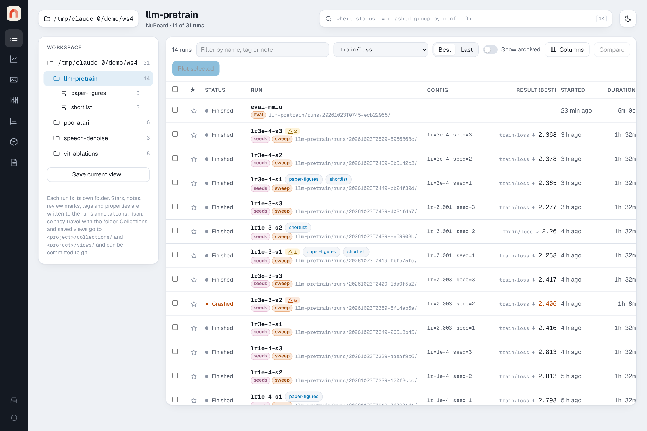
Header
- Folder chip: the served folder; click it to go back to all runs.
- Query bar (Ctrl/⌘+K): filters, groups and orders runs everywhere in the app. See the query language.
- Time zone chip (the clock button): Local time by default, which shows times as they always have been, in your computer's zone. Optionally, pick another zone to show every date and time in. See Time zones.
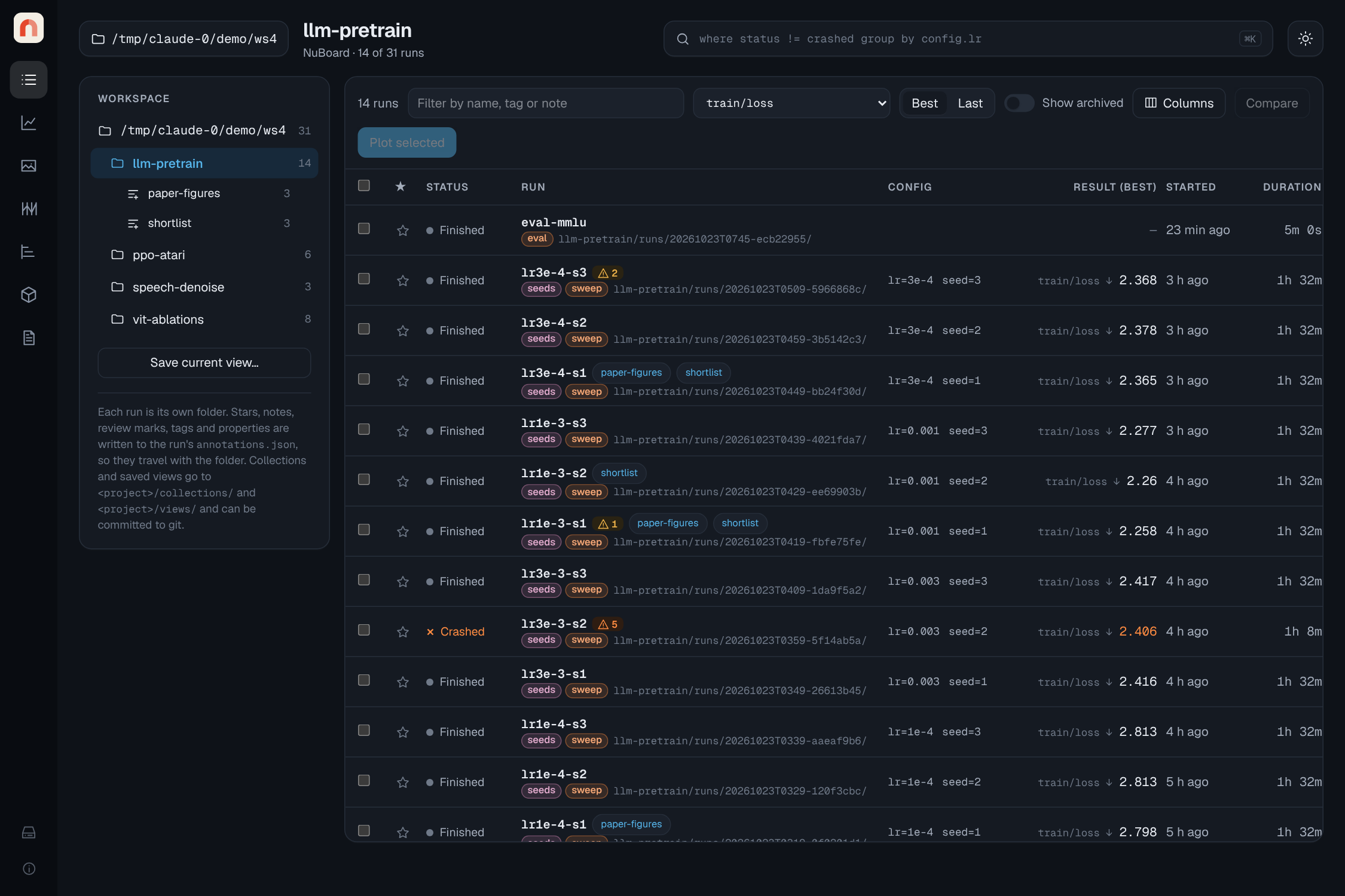
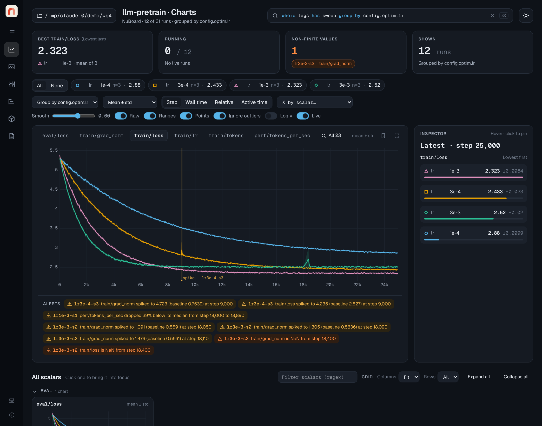
- Theme toggle: light and dark themes; the default follows your system.
- About (the small ⓘ at the bottom of the side bar): the version, the copyright, the license and a link to this documentation.
Runs page
- Workspace (left): every project found under the folder, with run counts,
its collections and its saved views. Save current view… writes the
current URL state to
<project>/views/<name>.json, which you can commit. Click a view to open it. The × that appears on hover deletes a view or a collection, after asking; the runs themselves are not touched. The button beside Workspace (or[) folds the list into a thin bar, which is remembered in this browser. - Table: status, star, name and folder (with the run's collections and its tags as colored pills; a tag keeps its color everywhere), the config keys that differ between the listed runs, a result column, start time, duration, reviewed mark and notes. Pick the result scalar in the toolbar and switch between Best (min for losses and errors, max otherwise) and Last. Click a column header to sort. The list is virtualized, so thousands of runs scroll smoothly.
- Filter box: quick text filter on name, id, project, tags and notes.
- Selection: tick runs to Star, Archive, Mark reviewed, edit their Tags, Properties or Collection, open them in Charts, Sweeps or Media, or Compare up to eight of them (the button reads Details with one run ticked, and opens its details). These actions sit in the blue selection bar, which appears once a run is ticked. Charts, Sweeps, Media and Timeline then show a Showing N selected runs banner with buttons to the other pages, which keep the selection, and Show all, which goes back to the query result; Clear selection ends it too.
- Alerts: a warning badge next to a run name counts its health alerts. Hover it to read them; click it to open the run's chart.
- Columns: add columns for any scalar (last value), any config key, or a property. The chosen columns are part of the URL.
- Notes: click a notes cell to edit it in place.
- Stars, notes, review marks, archive flags, tags edited in the viewer and
property values are written to
the run's own
annotations.json, so they move with the run folder. Archived runs are hidden unless Show archived is on. To delete runs, usenuboard rm.
Tags
Tags start as the ones passed to nb.init(tags=...) and can be changed in
the viewer at any time:
- In a run's details, the tag button next to its tags opens an editor: × removes a tag, and typing a name and pressing Enter adds one (tags used by other runs are suggested). Done or Esc closes it.
- To change many runs at once, select them and press Tags. Add takes tags separated by commas or spaces, and Remove lists the selected runs' tags to pick from. Each run keeps its other tags.
Once a run's tags are edited in the viewer, the edited list replaces the
logged one, so a tag set in nb.init can be removed too. The logged tags stay
in run.json as they were; the edited list is kept in annotations.json.
Properties
Properties are typed values you set on runs, such as a dataset, a verdict, an owner or a link to a paper. A property is defined once per project, with a type: text, number (with an optional unit), choice, tags, yes/no, date or link. Each run then has its own value, checked against that type.
- Define one: open Columns and press New property…, or press Add property in a run's Properties tab. Pick the name, the type, the options of a choice or tags property, and an optional description. From Columns the property is shown as a column right away, marked ✎.
- Set it on one run: click a cell in its ✎ column (Enter saves, Esc cancels, an empty value clears it), or edit it in the run's Properties tab.
- Set it on many runs: select them and press Properties. Pick the property, then its value, with a control that fits the type: buttons for a choice or yes/no, pills for tags, a date picker for a date. A name that is not defined yet is defined first.
Columns lists every property of the listed projects, to show or hide.
Values written without a definition, such as with Run.set_field from
Python, are marked Untyped; in a run's Properties tab, Untyped ·
define gives such a property a type.
Properties work in queries (verdict = "keep", score > 3,
topics has "augmentation") and as sweep parameters. From Python, read them
as run.fields and write them with run.set_field("verdict", "keep") in the
analysis API.
Collections
A collection is a named, hand-picked set of runs, such as a shortlist or the
runs behind a paper figure. Select runs and press Collection;
type an existing name to add to it. Collections are listed under their
project in the workspace; click one to filter to it (the query becomes
collections has "shortlist"), or hover it and press × to delete it (the
runs are not touched).
Each collection is a small JSON file, <project>/collections/<name>.json,
listing run ids, so it can be committed and survives moving the folder.
Run details and compare
Click a run name to open its details above the table, with the run's tags under its name (editable, see Tags): every setting (config, git commit, host, Python, GPUs, world size, fork origin, artifacts used and produced, last value of every scalar) and the run's files. A crashed run shows its traceback.
Console shows what the script printed, captured into files/output.log
by capture_console. It opens at the end,
like a terminal, shows the last 2 MB of a longer log, redraws progress bars
on one line and draws color codes as colors (the 16 terminal colors follow
the light or dark theme; 256-color and true-color codes, bold, dim, italic
and underline are drawn too). Raw shows the text as stored, with each
escape character as ␛. The file itself keeps the codes, so less -R in a
terminal shows the same colors.
Files lists everything in the run folder as a tree, with how many files
each folder holds and their size; files/ (what init and
add_file save, such as config.yaml, git.patch
and command.txt) starts open, other folders start folded. The tree is
about 12 rows tall and scrolls on its own; drag its corner to make it
taller. A long name loses its middle, so its end stays readable, and the
full path shows on hover. NuBoard's own data files (run.json,
data.parquet, event logs) are hidden until NuBoard data is switched
on. Pick a file to see it below the tree: text files are shown (diffed side
by side between two runs), images are drawn, and every file has a download
link. A text file with color codes or progress bars, such as a log, is
drawn like Console, with the same Raw switch, and diffed by its
visible text only.
Full screen shows a text file taller than its 520 px box on the whole
screen, scrolling inside; Exit full screen or Esc brings it back. A diff
keeps its Only changes switch and run menus there. A file that fits has no
button. While a run is running, its
open text file is read again as the run reports in, so a file it is still
writing grows in place: the scroll stays where you left it, and follows new
lines only when you are at the end.
Checkpoints (.pt, .pth, .ckpt, .bin, .safetensors, .npy,
.npz) list their keys as a tree with each tensor's shape, dtype and size,
and the total parameter count; with two runs the keys are diffed. Reading a
checkpoint needs no PyTorch and never runs code stored in it, and a file
that is cut off or malformed shows what could be read and why the rest
could not.
Pins turn files into tabs of their own, next to Files. The pin
button on a file (shown on hover) pins its path. A filter with * or ?
is a pattern over whole paths (* within a folder, ** across folders),
and Pin pattern pins it: checkpoints/*/best_*.pth shows each run's
own best checkpoint, newest first with a menu for the others, so runs whose
file names differ are still compared side by side. Pins are saved in
<project>/pins.json, so everyone viewing that data folder sees the same
tabs, in every run of the project; a pin only shows as a tab where a run has
a file it names. Unpin in a pinned tab, or the pin button in the tree,
removes it.
For a single run there are more tabs:
- Notes: Markdown notes for the run, with a preview. Notes can use
headings, lists, tables, links and code, and embed any logged item with
the same
line as a report. The runs table shows the first line; a note of more than one line opens here when clicked. - Properties: the run's properties. Add property defines one for
the whole project, with a type picked from a menu: text, number (with an optional unit),
choice, tags, yes/no, date or link. A choice is picked from a menu and tags
are toggled as colored pills; neither accepts a value outside its options,
which are added on purpose with New option… or + Option. Numbers,
dates and links are checked before saving, and the server rejects values
that do not fit (from the table, the API or
Run.set_fieldtoo). The bin button removes a property: its definition and its value on every run of the project. Values are saved in each run'sannotations.json, so they show up as columns and work in queries (verdict = "keep",topics has "augmentation"). Definitions are kept in<project>/fields.json. - Timing (only for a run with timers): where the run's
time went. A line on top gives the share of the run's wall time that timers
covered, the steps and the ranks, then a few findings, such as a step that
took over three times its timer's median, or a rank that was the slowest in
most steps; click a finding to show that step or every rank. The table lists
each timer with its Calls (
1.04Mfor a million), Mean/step, p95, Total, Share of the run and a line of its duration per step (hover for the value, click to show that step below; dashed lines mark resumed sessions). A timer whose spans fall inside another's is indented under it;summedmarks anaccumulate=Truetimer. Two more rows say how long ranks waited for each other and how much time no timer covered. Click a row for a full chart of that timer, and Open in Charts to compare it across runs. Timeline draws one step with a lane per rank: each span where it ran, summed timers as a thin strip (they have no position in time), and the time a rank waited for the others hatched;‹ ›moves between steps. Ranks switches between rank 0 and all ranks (per step the mean, shaded from the fastest to the slowest rank) or a single rank. Kept in the URL astrankandtstep.
The first five tabs show in the row; the rest are in the ⋮ menu at its end (the open tab always shows), so the row and the settings filter stay on one line on a laptop screen. The same menu has Charts, Sweeps and Media, which open those pages with only the run (or the compared runs), as the selection bar does, without ticking checkboxes.
With two to eight runs selected, Compare shows the same tabs side by side: All settings has a column per run and highlights rows where any run differs. Files and pinned tabs show a line diff between two of the runs. With more than two, pick which two from the Diff … against … menus. Only changes hides identical rows and lines.
The filter box above All settings narrows its rows by key, together with
Only changes, and shows how many keys are left (12 of 340 keys):
- Plain text matches part of a key, ignoring case:
edge.min,lr. - Text in slashes is a regular expression:
/^config\.generator\..*\.(min|max)$/. The .* button makes every term one. An invalid pattern turns the box red and leaves the list as it is. - A leading
!excludes keys, and terms separated by spaces must all match:generator !debug. - Values also matches the values, to find which keys are set to
adamw.
Matches are highlighted in the keys. / focuses the box and Esc clears it.
The filter is kept in the URL (sfind=), so it survives a reload and can be
shared.
Charts page
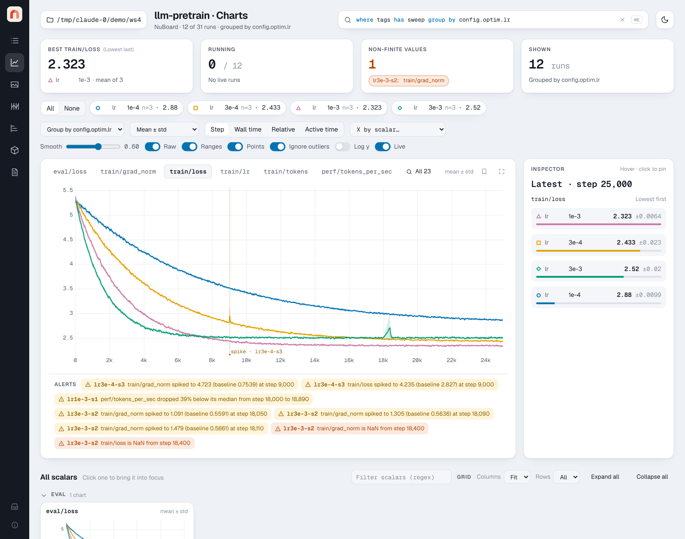
The Charts page plots the selected runs (from Charts in the selection bar) or, if none are selected, every run matching the query.
- Summary cards: best value of the focused scalar, running runs and last heartbeat, runs with NaN/Inf values, and how many runs are shown.
- Grouping:
group by config.optim.lrin the query (or the Group by menu) draws one line per group with a band: mean ± std (default), mean ± sem, mean with min–max, or median with min–max (aggin the query, or the band menu). Runs are interpolated onto a shared x grid on the server before aggregating, so runs with different logging steps combine correctly. Without grouping, each run is one line (up to 60; group to see more). - Logged ranges: a scalar logged with
lowandhigh(seeadd_scalar) is drawn with a shaded band around each run's line, smoothed along with it, and the inspector shows the range after the value. When runs are grouped, the band is the spread across runs instead. The Ranges switch (shown when a chart has bands) hides every band when they clutter the chart; it is kept in the URL asbands=0. - Baselines: a scalar with a reference value set with
add_scalar_baselineshows it as a dashed horizontal line, with a light band for its range. Runs with the same baseline (to 6 significant digits) share one gray line; a baseline only one run has is dashed in that run's color. Hiding a run hides its baseline, and highlighting a run highlights its baseline. Grouped charts draw the mean baseline of each group. The inspector lists each baseline with the runs it belongs to, the y-axis keeps every baseline in view, and the Baseline switch (shown when a run has one) turns them off. - Legend chips: hover to highlight a series, click to hide it, and double-click (or Alt-click) to show only that series; soloing it again shows them all. All and None before the chips show or hide every series, so you can start from None and click the few you want. Each series has a color and a marker shape, so series stay distinguishable without color.
- X axis: step, wall time, relative time since the run started, or active
time (relative time with pauses longer than five minutes removed). The
X by scalar menu plots against any other scalar instead, such as
train/tokensorepoch; counter-like scalars are listed first. The x scalar is matched to each point by step (interpolated when the two were logged at different steps), and zooming works as usual when the x scalar only grows. The choice is kept in the URL asx=metric:<name>. - Display row: Smooth and the Raw, Ranges, Points, Baseline, Ignore outliers and Log y switches sit on their own row under the grouping and x-axis controls.
- Smoothing: debiased exponential moving average (as in TensorBoard). With Raw on, the unsmoothed data is drawn faintly behind the smoothed line.
- Points: a dot on each curve at the logged point under the cursor, so
you can see where the real data points are (as in TensorBoard). When the
cursor is pinned (click the chart), the dots stay. Kept in the URL as
dots=0when off. - Ignore outliers (TensorBoard's "Ignore outliers in chart scaling"): fits the y-axis to the 1st–99th percentile of the values, so a few spikes (such as a huge loss at step 0) do not flatten every curve. Off, the axis fits every point. Log y switches to a log scale.
- Zoom and pan: drag across a chart to zoom into a range. Over the
focused chart, Ctrl (⌘ on a Mac) + scroll, or a trackpad pinch,
zooms in and out around the cursor, also past the ends of the data, with
the y-axis fitted to what is in view. Alt + scroll zooms both axes, as
in TensorBoard. Shift + drag pans in any direction, and Shift +
scroll pans along x. The server sends a finer resolution for the x range
(from the precomputed zoom levels in
data.parquet, or from the raw log for live runs) once you stop, with some data on each side so smoothing does not restart at the edge; the view stays where you left it while it loads. Double-click, or Reset zoom, to reset. - Inspector: hover a chart to see every series' value at that step, sorted best first, with ± std for grouped series. Click to pin the step. Without hovering it shows the latest values of the series shown (in the zoomed range).
- Linked crosshair: hovering any chart moves the crosshair on all of them.
- Full screen: the corner button above the focused chart (or Esc to leave) fills the screen with the chart and the inspector.
- Add to a report: the bookmark button above the focused chart saves it into a report, as it is shown: runs, grouping, smoothing, zoom and hidden series. The report draws it live and keeps a PNG copy for exports.
- All scalars: a small chart per scalar, grouped by prefix (
train/,eval/,perf/…). Small charts load as you scroll. Click a title to bring the scalar into focus. Hovering a small chart shows each run's value at the cursor, best first (up to eight, then "+N more"). While the main chart is pinned, every small chart draws a dashed line at that step with a dot on each curve, and hovering one shows its values there. The full scalar name is written under each chart; Full names in the display row turns that off (names=0). Grid sets the charts per row (fit to width, or 1 to 6) and the rows per section (1 to 6, or all); a section with more charts gets a pager. Both are remembered and kept in the URL (ccols,crows). Filter scalars takes a regular expression (as in TensorBoard, case insensitive;loss|acc,^train/) and shows only the matching charts; it is kept in the URL ascfind. The run's own scalars come last and start folded: system (system metrics) and then timing (timers, drawn with durations such as1.2 sor3m 05son the y axis and in the inspector, lower being better). Runs that renamed these prefixes withinit(system_prefix=..., timing_prefix=...)are handled the same way. - A run that logged NaN gets a dashed marker at the first NaN with a
NaN · runlabel. -
Live: while runs are running, the server pushes updates over Server-Sent Events and the charts redraw at most every two seconds. They hold still while you work with them: when the chart is zoomed, the cursor is pinned or you hover a chart, or when the Live switch is off, new points wait behind a New data · Update button. Hovering away from an unzoomed, unpinned chart draws them by itself.
-
Alerts strip: under the focused chart, the health alerts of the runs in view, leaving out runs switched off in the legend (a "+N in hidden runs" note counts them; click it to switch them back on). Click an alert to jump to it; spikes and drops are shaded on the chart.
Live updates
The server checks the folder every 1.5 s and pushes changes. The Runs page follows them as they come: values change in place, and rows do not move while the pointer is over the table. Open run details follow the run's status, duration and summary, and read the run once more when it finishes or crashes. Charts behave as described above. Media, Sweeps, Timeline, Artifacts and Reports do not change under you: when runs change, a New results · Refresh button appears next to the page title (changes that are only heartbeats are ignored). Going back to Runs or Charts catches up by itself.
Sweeps page
Parallel coordinates over the parameters that vary between runs, with brushing on every axis, a grid of scatters (one per parameter) and a best-runs table. The main chart can go full screen, and any plot can be added to a report. See Sweeps.
Timeline page
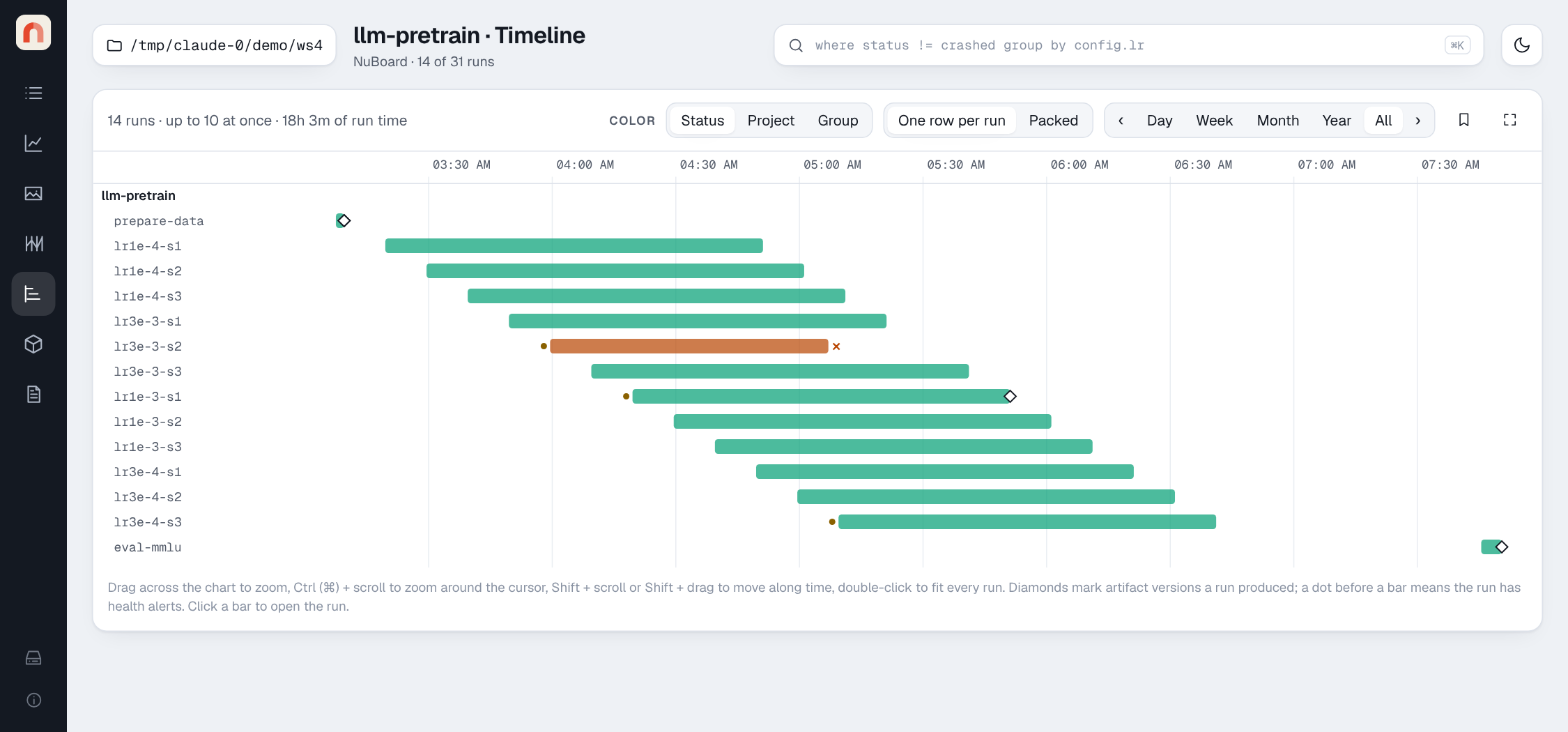
Every run as a bar from start to end, grouped by project, colored by status, project or group. Each row shows the run's name followed by the end of its id, which tells apart runs with the same name; hover a bar for the full id. Packed puts runs that never overlap on the same row, so the chart shows how many ran at once; the summary line gives the peak and the total run time. Crashed runs end in ✕, runs with alerts have a dot, and diamonds mark artifact versions a run produced. Click a bar to open the run.
To move around in time: Day, Week, Month and Year show that much time up to the latest activity, ‹ and › step one window back or forward, and All fits every run. Drag across the chart to zoom into a range, Ctrl (⌘) + scroll (or a pinch) zooms around the cursor, and Shift + scroll, a sideways scroll or Shift + drag moves along time. Double-click fits every run again. The axis switches to months and years for long ranges. The corner button shows the timeline full screen (Esc leaves), and the bookmark button adds it to a report as a snapshot.
Artifacts page
Every artifact version with its files, metadata and a lineage graph of the
runs that produced and used it. Started with --edit-artifacts, the page can
also add a version from a path and unlink or restore versions. See
Artifacts and lineage.
The disk button at the top of the list opens Storage on its
Artifacts tab.
Reports page
Lists the Markdown reports of every project, with an editor and a live preview side by side. See Reports.
Hypotheses page
A board per study of the hypotheses you tested, the runs that tested them and which run led to the next idea, drawn as a tree or a timeline. See Hypotheses.
Media page
Shows images, audio, video, figures, point clouds, HTML and text logged with
add_image, add_audio, add_video, add_figure, add_pr_curve, add_histogram, add_table,
add_point_cloud, add_html and add_text, for the selected runs (or
the query result, up to 48 runs). Each key is a collapsible section with a card
per run; every card has its own step slider, as in TensorBoard, so one run can
be scrolled through its steps while the others stay put.
- Runs: a chip per run, as in the Charts legend. Click one to hide or show it, double-click (or Alt-click) to show only that run, and All or None to show or hide every run.
- Kinds: the chips below (Images, Audio, Video, Figures, Tables, Point clouds, HTML, Text) show or hide a kind of media; double-click one to show only that kind. The number on each chip counts its keys.
- Filter keys: a regular expression on the keys, such as
^eval/orconfusion|per_class. While it is set, the count next to it shows how many keys match, and keys that do not match are hidden. - By key / by run: a section per key with a card per run (default), or a section per run with a card per key.
- Step: Latest shows each run's last item; Pick step moves every
card to the item at or before one step; Best scalar moves each run to
the item closest to the step where a scalar of your choice was lowest or
highest (for example the best
val/acc). Moving a card's own slider overrides the page-wide step for that card only. - Grid: Columns sets the cards per row (fit to width, or 1 to 8) and Rows how many rows each section shows per page (1 to 6, or all); a section with more cards gets a pager. Both are remembered.
- Expand all and Collapse all fold the sections; with many keys only the first three start open. Show runs without the key adds an empty card for runs that never logged it.
Each card can open its item large, download it, or add it to a report
(the bookmark button). Select for report adds a checkbox to every card
so several items go into a report at once; see Reports. The whole view is kept in
the URL (mkinds, mfind, mby, mmode, mstep, mmetric, mdir,
mcols, mrows), so a shared link shows the same grid.
Logged HTML runs in a sandboxed iframe (sandbox="allow-scripts", no
same-origin access) and is served with a matching Content-Security-Policy.
Output / code above it switches to the HTML source, with line numbers.
Matplotlib figures are stored as SVG and shown as images. Plotly, Vega-Lite
and Bokeh figures are interactive (hover, zoom, pan, export), each in its own
sandboxed iframe, and follow the light or dark theme. Every figure also has a
Download spec link for the raw JSON.
| Library | Rendered with | Network |
|---|---|---|
| Plotly | plotly.js 4, bundled with the viewer | none |
| Altair / Vega-Lite | Vega 6, Vega-Lite 6 and vega-embed, bundled | none |
| Bokeh | BokehJS from cdn.bokeh.org, for the exact version that wrote the figure |
needed when viewing |
nb.WaveformFigure |
uPlot, bundled (as on the Charts page) | none |
The bundled renderers load only when a figure of that kind is on screen. BokehJS has to match the Python Bokeh version, so it cannot be bundled; when the CDN is unreachable the figure shows a message and the spec stays downloadable.
Waveform figures
A waveform logged with add_figure(key, nb.WaveformFigure(audio, rate,
signals)) is drawn as a plot of the samples with each signal over it, accurate
at every zoom: each pixel column draws the first, smallest, largest and last
sample under it, recomputed as you zoom, so long files stay fast and single
samples show when zoomed in. Hovering shows the time, sample index and exact
values, and the label of each region track logged with the figure (drawn in
lanes under the plot, a row per class where classes overlap). Drag to select a
section, then loop it, zoom to it or add a Note; notes show in a lane above
the plot and are saved like audio notes. − / + / Fit, Ctrl/⌘ + wheel and
double-click zoom, Shift + wheel scrolls, and the overview below the plot moves
the view. The full screen button (next to Fit) spreads the figure over the
window with a taller plot, in the viewer and in exported reports alike; there
Space plays and pauses, and Esc puts it back. The play button plays the clip, or the selection, from where you
click. The download button next to it saves the Audio (.wav) as logged or
the Data (.zip): the audio, one .npy per signal and a metadata.json
(details). Other
items download from their card with an extension that matches their type
(.png, .wav, .json, ...). It has no spectrogram; Audio has that. See
add_figure.
Tables
Tables (add_table) take the whole width of the section. Each run's card has
its step slider, and every number is compared with the same row at the
Previous step or the First step (or Nothing): the cell is tinted
green when it got better and orange when it got worse, darker for bigger
changes, with the change next to the value (Color + Δ, Color or
Δ). A column counts as better when lower if its name looks like a loss or
error (loss, error, wer, ...), and when higher otherwise; the arrow next
to each column name says which.
- Click a column to sort; rows glide to their new place when the step changes, and the arrows next to the rank say how many places a row moved.
- Filter rows takes comparisons joined with
and, such assnr_in < 0 and noise = babble; other text matches the row id. - The summary counts the rows that improved or got worse on the sorted column (or the first column that changed), with its mean and change.
- Trend draws that column for each row across the logged steps.
- Click a row for its values at every step and its media: an audio cell opens in the waveform player, with notes.
In an HTML export a table shows its first 200 rows, colored by the change since the previous step.
PR curves
PR curves are listed with the figures. Each card draws its run's curve (precision against recall) in the run's color with its average precision (AP, the area under the curve, by the trapezoidal rule), and a chart above the cards overlays every run's curve at the chosen step, as TensorBoard does; its buttons open it large, download it as a PNG with its legend, or add it to a report. Hover a curve for the threshold, precision, recall and the TP, FP, TN and FN counts there.
Distributions
Distributions (add_histogram) are listed with the figures. Each card draws
its run's histogram at the chosen step, filled in the run's color, with the
step logged before it as a dashed outline, so you see how it moved. The y axis
is density, so steps and runs with different ranges or bin counts compare
fairly. Hover for the bin under the pointer and its share of the values.
Over steps switches the card to TensorBoard's distributions view: the
median as a line and bands holding 68%, 86% and all of the values at every
logged step (up to 150, sampled evenly), with the chosen step marked. A chart
above the cards overlays every run's histogram at the chosen step; its
buttons open it large, download it as a PNG with its legend, or add it to a
report. In an HTML
export a distribution is drawn as a picture with the step before it.
Point clouds
Point clouds are drawn in a view you can rotate (drag), pan (shift-drag or
right-drag), zoom (click the view, then scroll) and reset (double-click),
colored by their logged colors or else by height. Axes under the view
draws the x, y and z axes from the cloud's lowest corner, with round values
along them; they start shown when the cloud was logged with axes, labeled
with its names. Each card has its step
slider, so you can watch a cloud change over training; the zoomed view draws
it larger. The renderer is a few hundred lines of plain canvas code, so it
needs no WebGL and works the same in an HTML export.
Video
A clip logged from frames (add_video with an array)
plays in a frame player: play and pause, a slider to step through the frames
one at a time (it pauses playback), and the frame number and frame rate. It
loops, as TensorBoard's does. MP4, WebM, MOV and Ogg files play in the
browser's own video player, muted and looping, with its controls. Moving the
card's step slider shows the clip of another step, so you can watch a policy
or a generator improve over training.
Audio
Audio has two players, switched with Audio above the grid (the choice is remembered):
- Waveform (default): waveform and spectrogram of every channel, with a
minimap, time ruler, zoom (buttons, slider,
+/-, or Ctrl + wheel), drag-to-select with loop (L) and zoom-to-selection (Z), playback speed, and full screen (F), where Space plays and pauses. The spectrogram is computed in the browser (Hann window of 1024 samples, levels in dB relative to a full-scale sine on a fixed scale, so clips can be compared by eye). The players of one key follow each other's zoom, scroll, cursor and selection, and starting one pauses the others, so you can listen to the same passage across runs. Space plays and pauses; arrow keys seek. Next to the player switch, Colors picks the spectrogram colormap (theme, viridis, magma or gray), Frequency its scale (linear, log or mel), Window the FFT size (256 to 4096 samples; the hop is a quarter of it), and Spectrogram hides it to show only waveforms. Amplitude axis labels the waveform's amplitude (±1 is full scale) down its left edge. The choices are remembered in the browser and kept in the URL (cmap,fscale,fft,spec,amp), so a shared link shows the same view. - Simple: the browser's own audio controls, as in TensorBoard.
Notes: in the waveform player, select a section and press Note (or
N), type, and press Enter. Notes show in a lane above the waveform; click
one to select its section again, then Edit note changes or deletes it.
Notes are saved in the run's annotations.json (keyed by the media key and
step), so they show wherever the clip does, including reports, and an HTML
export lists them under the clip with buttons that play each section. From
Python, Run.audio_notes reads them.
Each clip shows its caption, duration, sample rate and channels, and a download link. The waveform player is a port of the player in audioviewer, built on wavesurfer.js (BSD-3), bundled with the viewer so it works offline.
Storage
The disk button at the bottom of the left rail shows how much disk the served folder uses, like a system storage panel. Nothing is measured until you press Measure, and the result stays until you press Refresh, with the time it was measured. It is kept across restarts of the viewer.
- Runs shows one bar for the whole folder, split into runs, artifacts and other files (reports, views, ...), then every project by size. Open a project to see its largest runs, each split into scalars, media, files and console output; click a run to open it.
- Artifacts lists each artifact with its versions. Only what is stored in the folder counts: a copied version counts its files, a referenced version only its manifest. The size a reference points to is shown apart, as "points to … elsewhere".
Measuring only lists folders and reads file sizes; it never opens a file, and a symlink counts as the link, not what it points to. On a very large folder it pauses after 10 s and asks whether to go on; Stop here keeps what was measured so far, marked as partial.
Time zones
Every time a run records is stored as Unix seconds, an exact moment that does not depend on any time zone. The viewer writes those moments in one zone. You never have to choose one: by default the chip in the header reads Local time, and times are shown as they always have been, in your computer's zone, with nothing converted (hover the chip to see which zone that is). To see times in another zone, click the chip and pick:
- Local time (the default): your computer's zone, no conversion.
- Machine time: each run on the clock of the machine that recorded it. See Machine time.
- UTC.
- A named zone, such as
America/SantiagoorEurope/Berlin. Type a city to find it. A named zone follows daylight saving at each moment: a run from January and one from July both show the clock time of their own season, no matter when you look at them. - A fixed offset, such as
UTC-03:00, which never changes. Type any offset betweenUTC-14:00andUTC+14:00.
The choice changes how times are written, and nothing else: data, queries
(started > … still compares Unix seconds), links and saved views stay the
same. It applies everywhere at once (the run table, run details, chart
tooltips and wall-time axes, the Timeline, artifact and file dates, and
exported reports), so the same moment always reads the same. Hover read-outs
end with the zone's short name, such as GMT-3. The choice is kept per
browser, so two people opening the same link each see their own zone. When a
picked zone differs from your computer's, the chip shows its short name and
place (GMT+1 Berlin) with a small dot. Pick Local time to go back.
Converting needs no network: browsers ship the time zone rules, with each zone's history, so past times stay right after a country changes its rules. Only a browser that has not been updated since a new rule took effect shows times after that change off by the difference; UTC and fixed offsets avoid zone rules altogether.
Machine time
With Machine time, every time that belongs to one run (the run table's
start time on hover, run details, the Timeline's hover card) is written on
the clock of the machine that recorded it, using the offset saved with each
session. A run resumed on another machine switches clock at the resume, such
as UTC−03:00 before it and UTC+01:00 after it.
A wall-time chart axis or the Timeline puts several runs on one axis, which can only have one clock. Where the points sit never changes (they are exact moments); only the labels do:
- When every run shown was recorded in the same zone, the axis uses it, and
the caption next to it reads
UTC−03:00 · machine time. - When they come from different zones, the axis and its read-out are in UTC,
and the caption reads
UTC · runs from different zones. Each run's own time is still in its run details and hover card. - When no run's zone is known, local time is used, captioned
local time, machine zone unknown.
A run whose machine zone is not known shows local time instead, marked
(local) after the time.
The machine's zone
Run details show a machine_zone row: the UTC offset of the machine
that recorded the run, and its host, such as UTC−03:00 · lab. A run
resumed later gets a row per extra session (machine_zone.s1, …), so a run
started in Santiago and resumed on a cluster in Europe reads UTC−03:00 ·
lab and UTC+01:00 · cluster. Each session records its own offset at start
and at finish, so a clock change during a session shows as
UTC−03:00 → UTC−04:00 (clock change). Hover a value for what it means.
Runs recorded before this was saved show the first session's offset worked
out from the run id (whose timestamp is the machine's local time at init),
dimmed, as ≈ UTC−03:00 (from run id). It is unknown when it cannot be
worked out: later sessions of those runs, runs given an explicit run_id,
and TensorBoard imports.
The zone setting corrects a machine set to another zone, not a machine whose clock is wrong: if a clock was off, the times it recorded are off too.
Sharing on a network
Sharing from a cloud machine compares the ways to reach a viewer on another machine (SSH port forwarding, a token, HTTPS behind a proxy) and what each means for access and security.
nuboard up --host 0.0.0.0 (or a specific address) makes the viewer reachable
from other machines, and anyone who reaches it could read your runs and change
notes, tags and reports. So, like Jupyter, it then asks for a token:
$ nuboard up ~/exp --host 0.0.0.0
nuboard serving ~/exp (31 runs) at http://gpu-box:6070/?token=3f9c…e1  (Ctrl+C to stop)
  Open the link above once per browser; it signs the browser in.
- Opening the link signs the browser in with a cookie for 30 days and removes the token from the address bar. Without it, pages show a sign-in form where the token can be pasted, and API calls get a 401.
- A new random token is made each start.
--token VALUEor theNUBOARD_TOKENenvironment variable sets a fixed one, so bookmarks keep working.--no-tokenturns it off, for a network you trust. - Scripts send
Authorization: token VALUE. - On
127.0.0.1there is no token, as before. You can still ask for one with--token.
Whatever the host, the viewer refuses changes that a page of another website tries to make through your browser.
The token travels in plain HTTP. On an untrusted network, keep the default
host and forward the port with ssh -L 6070:localhost:6070 gpu-box instead.
Artifacts stay read-only unless you add --edit-artifacts. Reports can be
edited and take uploads, and hypothesis boards can be edited, unless you add
--read-only-reports.