Get started

This page trains a small network and watches it train in NuBoard. The network learns to tell apart three interleaved spirals, which is quick to train on a laptop with nothing but NumPy. Along the way the run logs:

• the training and validation loss and accuracy, as scalars;
• a picture of the decision regions, as an image;
• a PR curve for each class;
• the distribution of the weights and their gradients;
• the hidden layer, projected to 3D, as a point cloud;
• a table following ten hard points through training.

The whole script is examples/get_started.py in the repository, shown in full at the end of this page. The snippets below are its important parts. Each call is described in full in the Python API.

Setup

pipuv

pip install nuboard

uv pip install nuboard   # or: uv add nuboard, in a uv project

It includes the viewer. Logging itself uses only the standard library, so a training script that logs never imports NumPy, PyArrow or the server.

The data and the model

Three spirals of 300 points each, shuffled and split into 720 points to train on and 180 to validate on:

rng = np.random.default_rng(seed)
x, y = spiral(300, rng)
order = rng.permutation(len(y))
x, y = x[order], y[order]
x_train, y_train, x_val, y_val = x[:720], y[:720], x[720:], y[720:]

The model is a network with one hidden layer of 64 ReLU units, trained with plain SGD in batches of 32. forward returns the hidden activations and the class probabilities, and backward returns the loss and the gradients. Any framework works the same way: NuBoard only sees the numbers and arrays you pass to it.

Start a run

nb.init creates the run, with its config and tags, and the with block finishes it at the end, or marks it crashed if the script fails:

import nuboard as nb

config = {"lr": lr, "hidden": hidden, "epochs": epochs, "batch_size": 32}

with nb.init("get-started", run_name=f"lr-{lr:g}", config=config, tags=["spiral"]) as run:
    ...

The run is written to experiments/get-started/runs/<id>/. Its config shows in the Runs table and can be queried, such as where config.lr > 0.1.

Log scalars

Log the loss of every batch with run.add_scalar, at a step that counts batches:

for i in range(0, len(y_train), 32):
    loss, grads = backward(params, x_train[i : i + 32], y_train[i : i + 32])

    for k in params:
        params[k] -= lr * grads[k]

    run.add_scalar({"train/loss": loss, "train/lr": lr}, step=step)
    step += 1

After each epoch, evaluate on the validation set and log at the step training reached, so both curves share an x axis:

hidden_val, probs = forward(params, x_val)
pred = probs.argmax(1)
val_loss = float(-np.log(probs[np.arange(len(y_val)), y_val] + 1e-9).mean())
run.add_scalar({"val/loss": val_loss, "val/acc": float((pred == y_val).mean())}, step=step)

run.add_scalar does not wait for the disk, so logging every batch costs microseconds. The part of each key before the / makes a section in the viewer: train and val.

Log media

Every five epochs, log what numbers alone do not show:

run.add_image("val/decision", decision_image(params, x_val, y_val), step=step)

for c, name in enumerate(CLASSES):
    run.add_pr_curve(f"val/pr/{name}", y_val == c, probs[:, c], step=step)

for k in ("w1", "w2"):
    run.add_histogram(f"params/{k}", params[k], step=step)
    run.add_histogram(f"grads/{k}", grads[k], step=step)

centered = hidden_val - hidden_val.mean(0)
pca = centered @ np.linalg.svd(centered, full_matrices=False)[2][:3].T
run.add_point_cloud(
    "val/hidden", pca, step=step, colors=PALETTE[y_val], axes=("PC 1", "PC 2", "PC 3")
)

run.add_table(
    "val/probe",
    [
        {
            "point": f"#{i}",
            "label": CLASSES[y_val[i]],
            "predicted": CLASSES[pred[i]],
            "p_label": float(probs[i, y_val[i]]),
            "radius": float(np.hypot(*x_val[i])),
        }
        for i in probe
    ],
    step=step,
)

• decision_image returns a (160, 160, 3) uint8 array, the predicted class over the plane with the validation points on top.
• A PR curve per class compares that class against the other two.
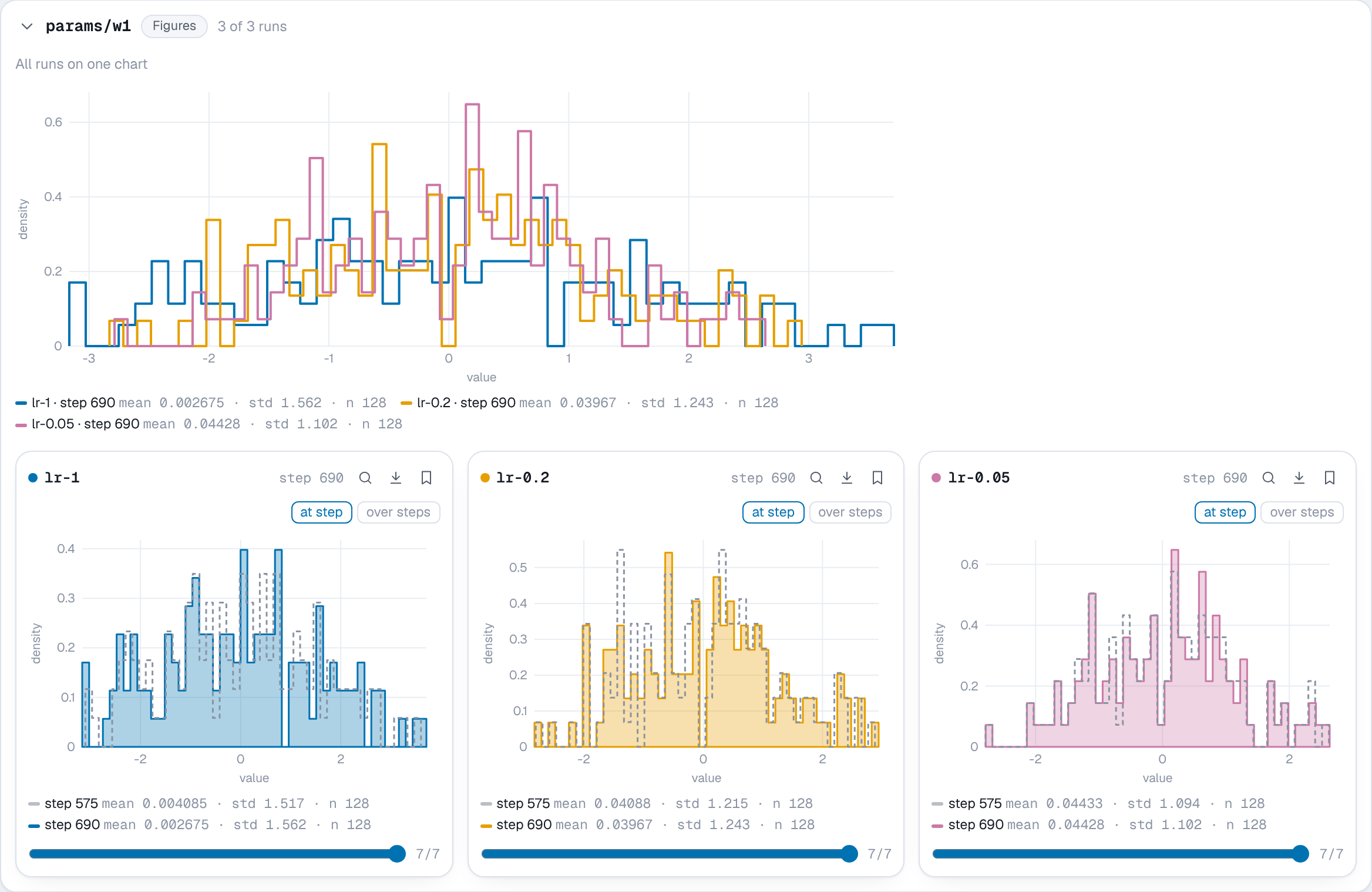
• The histograms show whether the weights grow and the gradients shrink.
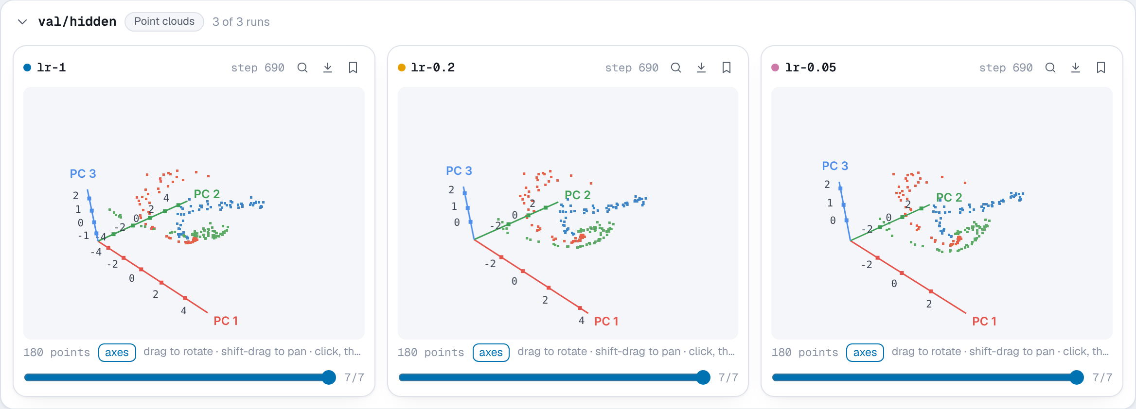
• The point cloud is the hidden layer reduced to three dimensions with PCA, colored by the true class. As the network learns, the classes pull apart.
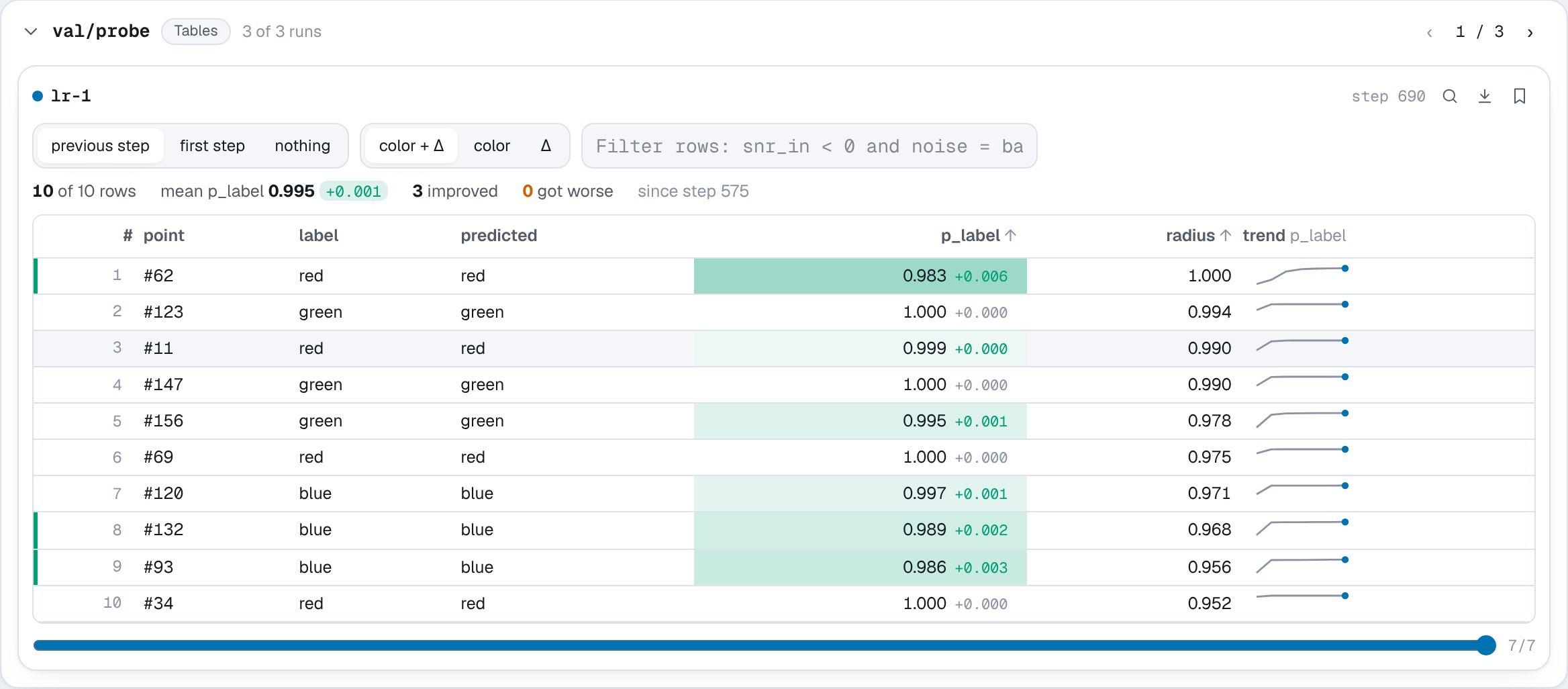
• The table logs the same ten points every time, the outermost ones, which are the hardest. The viewer matches rows by their first column, point, and shows how each one changed.

Train three learning rates

The script trains the same network with three learning rates, one run each:

for lr in (0.05, 0.2, 1.0):
    train(lr)

$ python examples/get_started.py
lr=0.05: val/acc 0.911, logged to experiments/get-started/runs/20261017T0932-71165378
lr=0.2: val/acc 0.978, logged to experiments/get-started/runs/20261017T0932-6c1850ee
lr=1: val/acc 1.000, logged to experiments/get-started/runs/20261017T0932-408224b6

Open the viewer

nuboard up experiments

and open http://localhost:6070. The viewer can also be started while training runs: it picks up new points every couple of seconds.

Runs

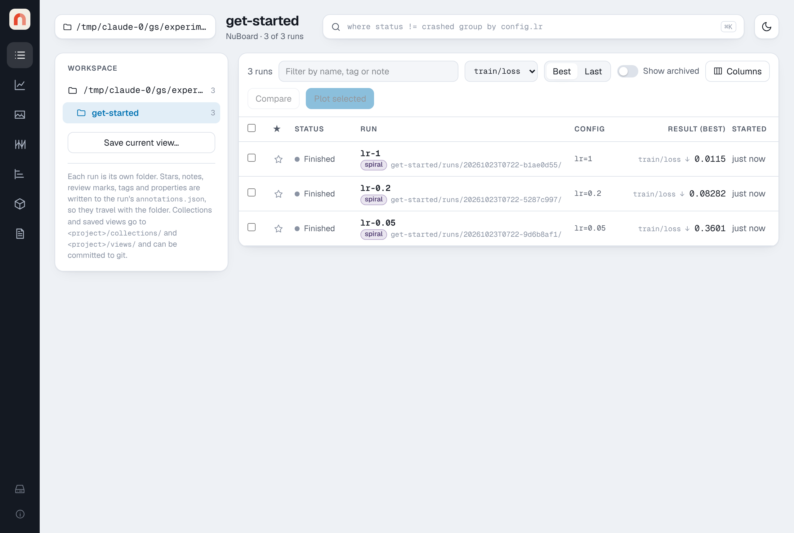
The Runs page lists the three runs with their config, tags, the result of a scalar you pick (here the best val/acc) and how long they took. Click a run's name for its details: the full config, git commit, installed packages and command line, recorded by nb.init.

Charts

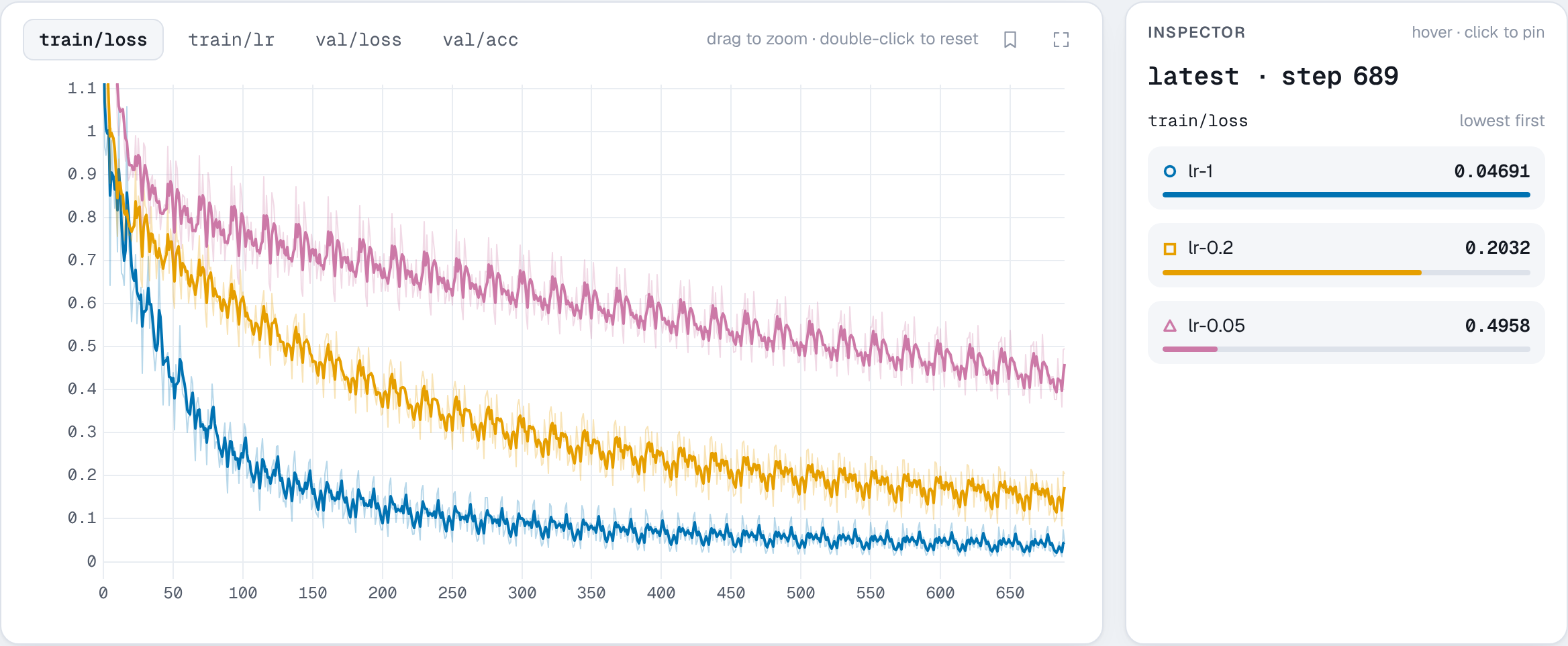
Select the three runs and press Charts in the selection bar. Each key is a chart with a line per run. The highest learning rate learns fastest here; the lowest has not converged after 30 epochs. Drag on a chart to zoom, and double-click to reset.

Media

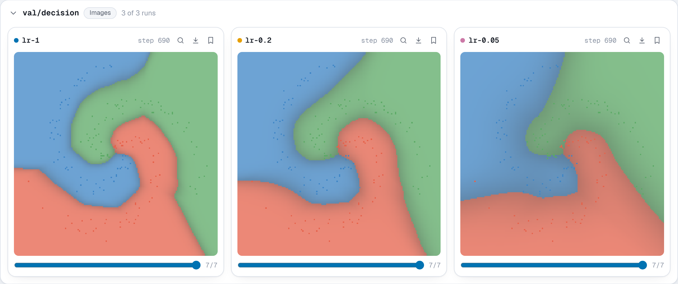
Media shows everything logged with add_*, a section per key and a card per run. Each card has its own step slider, so you can scroll one run through training while the others stay put.

The decision regions, at the last step, for the three runs:

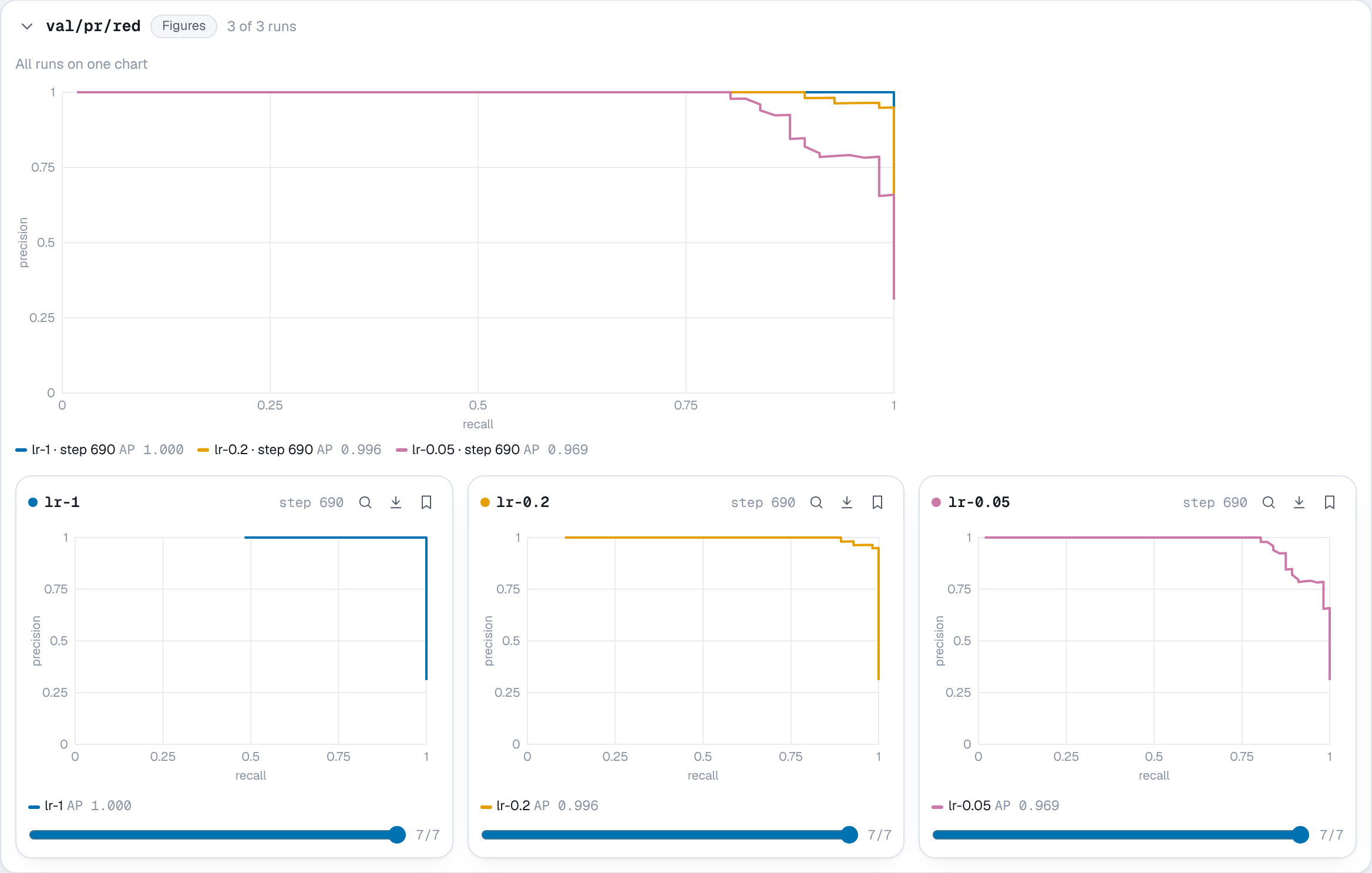
The PR curves of one class, overlaid for the three runs above the cards:

The weights of the first layer, at the last step against the step before it, and over steps:

The hidden layer of the best run, rotated with the mouse:

The probe table, with each cell tinted by how it changed since the step before:

What next

• The Python API describes every call, with the arguments it takes and what it stores.
• Using the viewer covers queries, grouping runs into mean and spread bands, comparing runs, properties and tags.
• Reports turn charts and media into a Markdown page you can export as one HTML file.
• Sweeps shows which hyperparameters matter.

The whole script

examples/get_started.py

"""Train a small NumPy network on a spiral and log it to NuBoard.

The script behind the Get started page of the docs. It needs only NumPy.

    python examples/get_started.py
    nuboard up experiments
"""

import numpy as np

import nuboard as nb

CLASSES = ["red", "green", "blue"]
PALETTE = np.array([[230, 97, 74], [92, 170, 102], [61, 133, 198]], np.uint8)


def spiral(n: int, rng: np.random.Generator) -> tuple[np.ndarray, np.ndarray]:
    """Return `n` points per class of three interleaved spirals, and their labels."""

    x, y = [], []

    for c in range(len(CLASSES)):
        r = np.linspace(0.05, 1, n)
        t = np.linspace(c * 4.2, (c + 1) * 4.2, n) + rng.normal(0, 0.25, n)
        x.append(np.stack([r * np.sin(t), r * np.cos(t)], 1))
        y.append(np.full(n, c))

    return np.concatenate(x), np.concatenate(y)


def init_params(rng: np.random.Generator, hidden: int) -> dict[str, np.ndarray]:
    """Return the weights of a 2-hidden-3 network with a ReLU, He-initialized."""

    return {
        "w1": rng.normal(0, np.sqrt(2 / 2), (2, hidden)),
        "b1": np.zeros(hidden),
        "w2": rng.normal(0, np.sqrt(2 / hidden), (hidden, 3)),
        "b2": np.zeros(3),
    }


def forward(p: dict[str, np.ndarray], x: np.ndarray) -> tuple[np.ndarray, np.ndarray]:
    """Return the hidden activations and class probabilities for `x`."""

    h = np.maximum(0, x @ p["w1"] + p["b1"])
    z = h @ p["w2"] + p["b2"]
    z = np.exp(z - z.max(1, keepdims=True))
    return h, z / z.sum(1, keepdims=True)


def backward(
    p: dict[str, np.ndarray], x: np.ndarray, y: np.ndarray
) -> tuple[float, dict[str, np.ndarray]]:
    """Return the cross-entropy loss on a batch and its gradients."""

    h, probs = forward(p, x)
    loss = float(-np.log(probs[np.arange(len(y)), y] + 1e-9).mean())
    dz = probs.copy()
    dz[np.arange(len(y)), y] -= 1
    dz /= len(y)
    dh = (dz @ p["w2"].T) * (h > 0)
    grads = {"w2": h.T @ dz, "b2": dz.sum(0), "w1": x.T @ dh, "b1": dh.sum(0)}
    return loss, grads


def decision_image(p: dict[str, np.ndarray], x: np.ndarray, y: np.ndarray) -> np.ndarray:
    """Return an HxWx3 picture of the predicted class over the plane, with the data."""

    size = 160
    g = np.linspace(-1.1, 1.1, size)
    grid = np.stack(np.meshgrid(g, -g), -1).reshape(-1, 2)
    _, probs = forward(p, grid)
    img = PALETTE[probs.argmax(1)].astype(float) * (0.35 + 0.4 * probs.max(1, keepdims=True))
    img = img.reshape(size, size, 3) + 255 * 0.25
    col = np.clip(((x[:, 0] + 1.1) / 2.2 * (size - 1)).round().astype(int), 0, size - 1)
    row = np.clip(((1.1 - x[:, 1]) / 2.2 * (size - 1)).round().astype(int), 0, size - 1)
    img[row, col] = PALETTE[y]
    return np.clip(img, 0, 255).astype(np.uint8)


def train(lr: float, hidden: int = 64, epochs: int = 30, seed: int = 0) -> None:
    """Train one network and log its run to the `get-started` project."""

    rng = np.random.default_rng(seed)
    x, y = spiral(300, rng)
    order = rng.permutation(len(y))
    x, y = x[order], y[order]
    x_train, y_train, x_val, y_val = x[:720], y[:720], x[720:], y[720:]
    config = {"lr": lr, "hidden": hidden, "epochs": epochs, "batch_size": 32}
    params = init_params(rng, hidden)
    probe = np.argsort(-np.hypot(*x_val.T))[:10]  # the outermost points, the hardest ones

    with nb.init("get-started", run_name=f"lr-{lr:g}", config=config, tags=["spiral"]) as run:
        step = 0

        for epoch in range(epochs):
            # 1. Train, logging the loss of every batch
            for i in range(0, len(y_train), 32):
                loss, grads = backward(params, x_train[i : i + 32], y_train[i : i + 32])

                for k in params:
                    params[k] -= lr * grads[k]

                run.add_scalar({"train/loss": loss, "train/lr": lr}, step=step)
                step += 1

            # 2. Evaluate once per epoch, at the step training reached
            hidden_val, probs = forward(params, x_val)
            pred = probs.argmax(1)
            val_loss = float(-np.log(probs[np.arange(len(y_val)), y_val] + 1e-9).mean())
            run.add_scalar(
                {"val/loss": val_loss, "val/acc": float((pred == y_val).mean())}, step=step
            )

            # 3. Media, every five epochs
            if epoch % 5 == 4 or epoch == 0:
                run.add_image("val/decision", decision_image(params, x_val, y_val), step=step)

                for c, name in enumerate(CLASSES):
                    run.add_pr_curve(f"val/pr/{name}", y_val == c, probs[:, c], step=step)

                for k in ("w1", "w2"):
                    run.add_histogram(f"params/{k}", params[k], step=step)
                    run.add_histogram(f"grads/{k}", grads[k], step=step)

                centered = hidden_val - hidden_val.mean(0)
                pca = centered @ np.linalg.svd(centered, full_matrices=False)[2][:3].T
                run.add_point_cloud(
                    "val/hidden",
                    pca,
                    step=step,
                    colors=PALETTE[y_val],
                    axes=("PC 1", "PC 2", "PC 3"),
                )

                run.add_table(
                    "val/probe",
                    [
                        {
                            "point": f"#{i}",
                            "label": CLASSES[y_val[i]],
                            "predicted": CLASSES[pred[i]],
                            "p_label": float(probs[i, y_val[i]]),
                            "radius": float(np.hypot(*x_val[i])),
                        }
                        for i in probe
                    ],
                    step=step,
                )

    print(f"lr={lr:g}: val/acc {float((pred == y_val).mean()):.3f}, logged to {run.path}")


if __name__ == "__main__":
    for lr in (0.05, 0.2, 1.0):
        train(lr)